
GO Faster Go Further
Established since 2001

Hydrogen Hot Rodding™ ©

Secure Supplies Group


Understanding Power Supply Designs
Forward Mode
Basic Forward Converter Mode
The VIC compared to a basic Forward Converter

Flyback Mode
Basic Flyback Converter Circuit
VIC comparison to the SMPS Flyback Converter

Suggested VIC circuit operation ON vs OFF states.

Linear Supplies
Linear Magneto Effect
The linear magnetoelectric effect in non-centrosymmetric magnetic insulators using a linear-response theory and the concept of magnetoelectric multipoles
ABSTRACT
We discuss the correspondence between the current-induced spin polarization in non-centrosymmetric magnetic metals and the linear magnetoelectric effect in non-centrosymmetric magnetic insulators using a linear-response theory and the concept of magnetoelectric multipoles. We show that the magnetoelectric toroidal moment is a particularly useful quantity since it determines the ground-state antiferromagnetic domain of a non-centrosymmetric antiferromagnet in the presence of a steady-state electric current. We analyze two prototypical antiferromagnetic spintronic materials—Mn2Au and CuMnAs—and show that the experimentally reported domain reorientations are consistent with the alignment of their toroidal moments parallel to the applied electric current. Finally, we determine whether similar behavior should be expected in the prototypical insulating magnetoelectric materials, Cr2O3 and Li𝑀PO4, if they could be doped into a semiconducting or metallic regime.
I. INTRODUCTION
A. The linear magnetoelectric effect
The linear magnetoelectric (ME) effect is the linear response of the magnetization of a material to an applied electric field, 𝜇0𝐌𝑗=𝛼𝑗𝑖𝐄𝑖, or the corresponding electric polarization induced by a magnetic field, 𝐏𝑖=𝛼𝑖𝑗𝐇𝑗,1 where 𝛼𝑖𝑗 is the magnetoelectric tensor.
It is caused by, for example, an electric field changing the angles and distances, and hence the magnetic exchange interactions, between magnetic ions,2 or a magnetic field reorienting spin magnetic moments, causing a change in the electronic charge density via the spin–orbit coupling.3,4 Notably, it allows for reorientation of antiferromagnetic domains by the simultaneous application of magnetic and electric fields, with potential device applications in electrical control of exchange bias.5 A requirement for its occurrence is the absence of both space-inversion and time-reversal symmetry, and it is formally defined only in insulating systems because metals screen an applied electric field and their electric polarization is ill-defined.
B. Current-induced spin polarization
While an electric field cannot cause a linear magnetoelectric response in magnetic metals, an electric current can modify their magnetism.
One mechanism by which this is proposed to occur is the so-called spin–orbit torque effect, in which spin angular momentum is transferred from the conducting electrons to the constituent magnetic ions through their spin–orbit coupling. There has been considerable excitement following reports of such a mechanism causing rotation of the antiferromagnetic vector in metallic antiferromagnets,6,7 suggesting future antiferromagnetic spintronic device applications. A requirement for a current-induced rotation of a spin is that the space-inversion symmetry is broken locally at its magnetic site, reminiscent of the symmetry requirement for the magnetoelectric effect in insulators.8
C. Link between electric field- and electric current-induced magnetization
In this work, we clarify the relationship between the current-induced spin polarization in a metal and the linear magnetoelectric response in an insulator.
We begin by showing the formal correspondence between the two phenomena using linear-response theory. We then introduce the concept of magnetoelectric multipoles, which has proved useful in the magnetoelectric community, and show that it can also be a convenient formalism for discussing current-induced spin polarization. To illustrate the connection, we calculate the magnetoelectric multipoles in the prototypical spin–orbit torque metals, Mn2Au and CuMnAs, and discuss their possible relevance for both switching and stability of the antiferromagnetic domains. Finally, we discuss whether the introduction of carriers into the prototypical insulating magnetoelectrics will lead to any interesting current-induced effects.
II. THEORETICAL CORRESPONDENCE
A. Linear-response description of linear magnetoelectricity and current-induced spin polarization
We begin by reviewing the linear-response theory descriptions of both linear magnetoelectricity and current-induced spin polarization, both of which have been treated previously (although separately) in the literature. This formalism immediately reveals a similarity between the two phenomena, as well as important differences.
1. Linear-response theory of the magnetoelectric effect
An explicit expression for the magnetoelectric susceptibility can be derived either from the Berry phase theory of polarization using 𝜒𝑖𝑗=∂𝑃𝑖∂𝐵𝑗|||𝐵→0,9 or within the Kubo linear-response framework.10,11 In both cases, one obtains the following expression for the spin contribution to the magnetoelectric susceptibility,
𝜒ME𝑖𝑗=𝐶Im∑𝐤,𝑚≠𝑛𝑓𝑛𝐤−𝑓𝑚𝐤(𝐸𝑛𝐤−𝐸𝑚𝐤)×⟨𝜓𝑛𝐤|𝑆̂ 𝑖|𝜓𝑚𝐤⟩⟨𝜓𝑚𝐤|𝑣̂ 𝑗|𝜓𝑛𝐤⟩(𝐸𝑛𝐤−𝐸𝑚𝐤).
(1)
Here, 𝑚 and 𝑛 are band indices, 𝐤 are reciprocal space vectors, 𝐸𝑛𝐤 are the band energies of the spinor Bloch functions 𝜓𝑛𝐤 with Fermi–Dirac occupations 𝑓𝑛𝐤, and 𝑆̂ and 𝑣̂ are the spin and velocity operators. In this formulation, the magnetoelectric susceptibility tensor 𝜒ME=∂𝐏/∂𝐁=∂𝐌/∂𝐄 has units of conductance (A/V), which is particularly convenient for the comparison with current-induced spin polarization. (The conventional definition used in the magnetoelectrics community is 𝛼=∂𝐏/∂𝐇=𝜇0∂𝐌/∂𝐄, in which 𝛼 has units of s/m.)
2. Linear-response theory of current-induced spin polarization
Following Ref. 12, we take the usual approach of writing the current-induced spin polarization, 𝛿𝐒𝑖, as 𝛿𝐒𝑖=𝜒𝑖𝑗𝐄𝑗, where 𝐄𝑗 is the electric field. We note, however, that the field in this case is produced by a current, whose symmetry properties are different from those of an electric field. The susceptibility 𝜒𝑖𝑗 is then obtained from the Kubo linear-response framework as8,12–14
𝜒𝑖𝑗=𝐶∑𝐤,𝑚≠𝑛⟨𝜓𝑛𝐤|𝑆̂ 𝑖|𝜓𝑚𝐤⟩⟨𝜓𝑚𝐤|𝑣̂ 𝑗|𝜓𝑛𝐤⟩𝐸𝑛𝐤−𝐸𝑚𝐤+𝑖Γ𝑓𝑛𝐤−𝑓𝑚𝐤𝐸𝑛𝐤−𝐸𝑚𝐤,
(2)
where Γ describes the effects of band broadening arising from a finite temperature or disorder and the other symbols are as defined in Eq. (1). The response can be separated into an intraband Fermi surface contribution, and two so-called interband contributions that depend on all of the bands, one of which is intrinsic and one that is caused by disorder. These have the following form:12
Fermi surface term
𝜒I𝑖𝑗=−𝐶2Γ∑𝐤,𝑛⟨𝜓𝑛𝐤|𝑆̂ 𝑖|𝜓𝑛𝐤⟩⟨𝜓𝑛𝐤|𝑣̂ 𝑗|𝜓𝑛𝐤⟩×𝛿(𝐸𝑛𝐤−𝐸𝐹).
(3)
The 𝛿(𝐸𝑛𝐤−𝐸𝐹) factor means that only states at the Fermi surface contribute to 𝜒I.
Intrinsic bulk term
𝜒IIa𝑖𝑗=𝐶∑𝐤,𝑛,𝑚Im⟨𝜓𝑛𝐤|𝑆̂ 𝑖|𝜓𝑚𝐤⟩⟨𝜓𝑚𝐤|𝑣̂ 𝑗|𝜓𝑛𝐤⟩×Γ2−(𝐸𝑛𝐤−𝐸𝑚𝐤)2((𝐸𝑛𝐤−𝐸𝑚𝐤)2+Γ2)2(𝑓𝑛𝐤−𝑓𝑚𝐤).
(4)
This contribution depends on all occupied and unoccupied bands; in the zero kelvin limit, the contributions of the Fermi–Dirac occupation factors split the sum into matrix elements between occupied and unoccupied states.
Disorder-induced bulk term
𝜒IIb𝑖𝑗=2𝐶∑𝐤,𝑛,𝑚Re⟨𝜓𝑛𝐤|𝑆̂ 𝑖|𝜓𝑚𝐤⟩⟨𝜓𝑚𝐤|𝑣̂ 𝑗|𝜓𝑛𝐤⟩×(𝐸𝑛𝐤−𝐸𝑚𝐤)Γ((𝐸𝑛𝐤−𝐸𝑚𝐤)2+Γ2)2(𝑓𝑛𝐤−𝑓𝑚𝐤).
(5)
Again, this contribution depends on all occupied and unoccupied bands. For the case of a perfect crystal without disorder at zero temperature, Γ→0 and the contribution from Eq. (5) is zero.
In an insulating material, there is no Fermi surface and as a result no contribution of the form of Eq. (3). As mentioned above, in a material with no disorder, Γ=0, and there is no contribution of the form of Eq. (5). Therefore, in the limit of an insulating system with no disorder, the susceptibility reduces to
𝜒𝑖𝑗=𝐶∑𝐤,𝑚≠𝑛Im⟨𝜓𝑛𝐤|𝑆̂ 𝑖|𝜓𝑚𝐤⟩𝜓𝑚𝐤|𝑣̂ 𝑗|𝜓𝑛𝐤×𝑓𝑛𝐤−𝑓𝑚𝐤(𝐸𝑛𝐤−𝐸𝑚𝐤)2.
(6)
We see that the expression is identical to that for the magnetoelectric susceptibility in Eq. (1).
B. Magnetoelectric multipoles
A concept that has proved useful in the theory of linear magnetoelectrics is that of the so-called magnetoelectric multipoles, which form the second-order term, 𝐸(2)int, of the multipole expansion of the free energy density of a magnetization density 𝐌(𝐫) interacting with an inhomogeneous magnetic field 𝐁(𝐫),15–18
𝐸(2)int=−∫𝑟𝑖𝑀𝑗(𝐫)∂𝑖𝐵𝑗(𝐫)𝑑3𝐫=−ℳ𝑖𝑗∂𝑖𝐵𝑗(𝐫)=−𝑎(∇⋅𝐁)−𝐭⋅(∇×𝐁)−𝑞𝑖𝑗(∂𝑖𝐵𝑗+∂𝑗𝐵𝑖).
(7)
Here, ℳ𝑖𝑗=∫𝑟𝑖𝑀𝑗(𝐫)𝑑3𝐫 is the nine-component magnetoelectric multipole tensor, which can be decomposed into the magnetoelectric monopole per unit volume, 𝑎=13∫𝐫⋅𝐌(𝐫)𝑑3𝐫, the toroidal moment per unit volume, 𝐭=12∫𝐫×𝐌(𝐫)𝑑3𝐫, and the magnetic quadrupole per unit volume, 𝑞𝑖𝑗=12∫[𝑟𝑖𝑀𝑗+𝑟𝑗𝑀𝑖−23𝛿𝑖𝑗𝐫⋅𝐌(𝐫)]𝑑3𝐫. (𝐸(1)int=−𝐌⋅𝐁, where 𝐌=∫𝐌(𝐫)𝑑3𝐫, would be the usual dipolar contribution to the free energy density.) Note that, for systems with no net magnetization such as the antiferromagnets considered in this work, the magnetoelectric multipoles are independent of the choice of the origin used in evaluating them.19
An insulator whose only non-zero magnetoelectric multipole is a monopole has a diagonal, isotropic magnetoelectric response,17 while a toroidal moment yields an antisymmetric magnetoelectric response19 and a quadrupole moment a symmetric, traceless response.
This multipole formalism has proved useful in designing new magnetoelectric materials based on their spin magnetization densities,2 as well as in the development of expressions for calculating magnetoelectric coupling parameters from first-principles.18,20 Both local magnetoelectric multipoles (analogous to local magnetic moments at the magnetic dipole level) and bulk thermodynamic quantities (analogous to the bulk magnetization density at the magnetic dipole level) have been defined.
The latter describe the global magnetoelectric response of the material, the former the local response at each atom to an external field. Intriguingly, it was recently demonstrated that magnetoelectric multipoles also exist in metals of an appropriate symmetry and that their magnitudes can be similar to those of typical magnetoelectric insulators, even though a conventional magnetoelectric response is not possible.21
A link can be made between the magnetoelectric multipoles and the linear-response susceptibility by noting that the nine-component tensor ℳ𝑖𝑗=∫𝑟𝑖𝑀𝑗(𝐫)𝑑3𝐫, of which the monopole, toroidal moment and quadrupole are irreducible components, describes the linear response of the energy to spatial variations in the magnetic field. Therefore, it can be written in terms of derivatives of the free energy density with respect to the corresponding derivatives of the field gradient as
ℳ𝑖𝑗=−lim𝐁(𝐫)→0∂𝐸(2)int(𝐫)∂(∂𝑖𝐵𝑗)|||||𝐁(𝐫).
(8)
Gao et al.20 used semiclassical electron dynamics theory to show that, for the spin component of the response in a periodic solid, this magnetoelectric multipole density tensor takes the form
ℳ𝑖𝑗=−𝐶Im∑𝐤,𝑚≠𝑛(𝐸𝑛𝐤+𝐸𝑚𝐤−2𝜇)𝑓𝑛𝐤−𝑓𝑚𝐤(𝐸𝑛𝐤−𝐸𝑚𝐤)2×⟨𝜓𝑛𝐤|𝑆̂ 𝑖|𝜓𝑚𝐤⟩⟨𝜓𝑚𝐤|𝑣̂ 𝑗|𝜓𝑛𝐤⟩,
(9)
where 𝜇 is the chemical potential. (Note that Ref. 20 refers to the magnetoelectric moment density ℳ𝑖𝑗 as the quadrupole; to avoid confusion with the quadrupolar component 𝑞𝑖𝑗, we prefer to avoid this terminology.) From this expression, it is clear that the magnetoelectric susceptibility and in turn the intrinsic bulk contribution to the current-induced spin polarization is obtained from the derivative of the magnetoelectric moment density with respect to the chemical potential, 𝜇,
𝜒𝑀𝐸𝑖𝑗=−𝑒∂ℳ𝑖𝑗∂𝜇.
(10)
Motivated by this correspondence between the descriptions of the susceptibilities describing the magnetoelectric and spin–orbit torque effects, we next use density functional theory (DFT) to quantify the link between them. First, we analyze the prototypical spin–orbit torque materials, Mn2Au and CuMnAs, for which the current-induced magnetic susceptibility has been well studied, in the context of the magnetoelectric multipoles.
Then, we discuss the prototypical magnetoelectric material, Cr2O3, for which the electric-field-induced magnetoelectric response and magnetoelectric multipoles are well known, and analyze its behavior when it is doped to support an electric current.
III. COMPUTATIONAL DETAILS
We perform density functional calculations using the VASP code22,23 (version 5.3.5) with projector-augmented wave (PAW) potentials24 and explicit inclusion of spin–orbit coupling. All calculations are performed at the experimental lattice constants and atomic positions taken from Ref. 25 for Mn2Au and Ref. 26 for CuMnAs.
For Mn2Au, we use an energy cutoff of 650 eV and a Monkhorst–Pack k-point grid27 of 12×12×6 for the conventional unit cell, which includes two formula units of Mn2Au. For Au, we use the “Au” default VASP PAW potential with 6𝑠15𝑑10 electrons in the valence. For Mn, we use the “Mn_sv” PAW potential with 3𝑠23𝑝64𝑠13𝑑6 electrons in the valence. We treat the exchange-correlation potential within the local density plus Hubbard 𝑈 approximation (LDA+𝑈)28 with 𝑈=4.63eV and 𝐽=0.54eV on the Mn atom.12
For CuMnAs, we treat the exchange-correlation within the local density approximation (LDA) and use an energy cutoff of 550 eV and a Monkhorst–Pack k-point mesh of 8×8×6. For Mn, we use the same “Mn_sv” potential as for Mn2Au and the “Cu_pv” (with 17 valence electrons) and default As (with 5 valence electrons) PAW potentials.
Local atomic-site magnetoelectric multipoles are computed through the decomposition of the atomic-site density matrix into irreducible spherical tensor moments,17,29 using the density matrix obtained using VASP.
IV. SPIN–ORBIT TORQUE MATERIAL EXAMPLES
Next, we discuss the two prototypical materials that have been used in studies of current-induced spin polarization, Mn2Au and the tetragonal variant of CuMnAs, which can be favored over the bulk orthorhombic structure using molecular beam epitaxial growth on GaAs or GaP.26 Their crystal structures and magnetic orderings are shown in Figs. 1 and 2.
Both are crystallographically centrosymmetric, with tetragonal symmetry so that the in-plane 𝑥 and 𝑦 axes are equivalent. When they order antiferromagnetically (Mn2Au at 𝑇𝑁≈1500K30 and CuMnAs at 𝑇𝑁≈480K31), the pattern of magnetic ordering breaks the inversion symmetry. For both materials, the antiferromagnetism is collinear, with easy-plane anisotropy, forming ferromagnetic layers in the 𝑎–𝑏 plane with antiferromagnetic stacking in the 𝑐 direction.30,31
This results in four energetically equivalent distinct antiferromagnetic domains, corresponding to in-plane rotations of the antiferromagnetic vector by 90∘. For CuMnAs, neutron diffraction shows that the 𝑥 and 𝑦 directions are the easy axes;31 therefore, in the magnetic ground state, which has a point group 4/𝑚𝑚𝑚, bulk (as well as local Mn) magnetoelectric moments of either 𝑡𝑦 and 𝑞𝑥𝑧 (for spins along [100]) or 𝑡𝑥 and 𝑞𝑦𝑧 (for spins along [010]) are allowed. For Mn2Au, density functional calculations7 show that the in-plane anisotropy is small and suggest the in-plane diagonals as easy directions.
For this spin orientation, and indeed for antiferromagnetic alignment along any general direction in the 𝑎–𝑏 plane, the magnetic point group is 2′/𝑚, which allows the bulk (and local Mn) magnetoelectric toroidal moments 𝑡𝑥, 𝑡𝑦, and the quadrupoles 𝑞𝑦𝑧, 𝑞𝑥𝑧, while all other local magnetoelectric multipoles are zero.
Our DFT calculations at the experimental lattice parameters and atomic positions yield antiferromagnetic orderings consistent with the literature, with Mn magnetic dipole moments of ±4.1𝜇𝐵 oriented along the [110] direction for Mn2Au and ±3.4𝜇𝐵 along the Cartesian axes for CuMnAs.
figure
FIG. 1. Crystal structure of Mn2Au. The unit cell is shown in black. The magnetic moments, oriented along the [110] direction, are shown with red arrows.
PPT|High resolution
figure
FIG. 2. Crystal structure of CuMnAs. The unit cell is shown in black. The magnetic moments, oriented along the [010] direction, are shown with red arrows.
PPT|High resolution
In both materials, application of a current pulse parallel to the spin-orientation direction results in a change of anisotropic magnetoresistance that is consistent with a reorientation of the spins to the direction perpendicular to the current.6,7
The spin reorientation has been explained by a spin–orbit torque mechanism caused by the 𝜒I component of the susceptibility,12 in which an in-plane current induces in-plane forces on the Mn ions, in such a way that oppositely oriented spin moments experience forces in opposite directions. As a result, the spins maintain their antiferromagnetic alignment to each other while they rotate away from the current direction.
Recently, however, a number of other proposals have emerged for the origin of the change in anisotropic magnetoresistance, including thermal effects32 and current-induced fragmentation of the antiferromagnetic domains.33 In addition, 180∘ current-induced switching of the spins, which would not be consistent with the simple spin–orbit torque mechanism, has been reported.34
A. Antiferromagnetic domain stability in the presence of an electric current
We begin by discussing how the concept of the toroidal moment introduced above is convenient in understanding how a steady-state electric current can lift the degeneracy between otherwise energetically equivalent antiferromagnetic domains.
Specifically, in the cases of Mn2Au and CuMnAs, the domain whose toroidal moment is parallel to the current is favored over the other three, whose toroidal moments are anti-parallel or perpendicular to the current direction. We emphasize that this is a feature of a steady-state current and does not describe the dynamics of a current pulse.
In Ref. 35, symmetry arguments were presented to demonstrate that the electric current, 𝐣, is the conjugate field for the toroidal moment, 𝐭. This means that in materials that possess a net toroidal moment—so-called ferrotoroidic materials16,19—the degeneracy of antiferromagnetic domains with different toroidal moments is lifted in the presence of an electric current, with the domain whose toroidal moment is parallel to the current being lowest in energy. (For a more detailed analysis, and group-theoretical classification of representative materials, see Ref. 36.)
The overall toroidal moment in a material with an antiferromagnetic arrangement of magnetic spins can usually be obtained straightforwardly by summing the cross product of the spins, 𝐬𝑖, multiplied by their positions, 𝐫𝐢,
𝐭∝Σ𝑖𝐫𝑖×𝐬𝑖
(11)
(for a discussion of subtleties that can sometimes arise due to the periodic boundary conditions see Ref. 19). For the CuMnAs unit cell shown in Fig. 2, in which the spins in the lower part of the unit cell are oriented along +𝑦 and those in the upper part along −𝑦, Eq. (11) yields a toroidal moment of size 0.4𝐒 along the +𝑥 direction, where 𝐒 is the size of the spin magnetic dipole moment on the Mn ion. Therefore, this spin structure is stabilized by a current along +𝑥, perpendicular to the spin orientation.
A current applied parallel to this spin arrangement will disfavor this domain relative to that with the spins rotated by 90∘, with currents along +𝑦 and −𝑦 promoting the two different domains in which the spins are aligned along the 𝑥 axis. (For cartoons indicating the four possible antiferromagnetic domains in CuMnAs, their corresponding toroidal moments, and the corresponding conjugate current direction, see Ref. 35.)
For the case of Mn2Au with the spin arrangement shown in Fig. 1, Eq. (11) yields a toroidal moment of size 2√3𝐒 along the [11¯0] direction, and therefore, this domain orientation is stable in a steady-state current along [11¯0].
As in the case of CuMnAs, a current parallel to the spin direction will increase the energy of the domain and favor a domain with perpendicular spin alignment, with opposite directions of the current favoring the domains with opposite antiferromagnetic vectors. Note that experiments have also been performed in which currents are applied along one of the Cartesian axes of Mn2Au. For this geometry, the lowest energy spin orientation from the point of view of the interaction energy between the toroidal moment and the current will again have its spins along the Cartesian axis that is perpendicular to the current.
Such a spin orientation is not in this case a ground-state configuration of the unperturbed system but could be stabilized by a sufficiently high current and small magnetic anisotropy energy.
We see that this simple analysis of the toroidization of an antiferromagnetic metal provides a convenient route to quickly determining the existence and orientations of current-induced selection of antiferromagnetic domains.
B. DFT calculations of local magnetoelectric multipoles and their change during spin rotation
Next, we analyze how the local multipoles on the Mn ions change during the switching process. We start by calculating the local magnetoelectric multipoles on the Mn ions in both Mn2Au and CuMnAs at the experimental lattice parameters and atomic positions in their ground-state antiferromagnetic structures that we calculated above.
The non-zero magnetoelectric multipole values that we obtain are listed in Table I and are consistent with the symmetry analysis that we presented above. Note that, for both materials, Mn ions of opposite spin directions have the same signs of their toroidal and quadrupole moments, indicating that while both materials are antiferromagnetic, they are both ferrotoroidal and ferroquadrupolar. In both cases, the local toroidal moments are oriented along axes that are perpendicular and crystallographically equivalent to the axis adopted by the spin magnetic dipoles.
The toroidal moment values for Mn2Au are slightly larger than those for CuMnAs for the same choice of pseudopotentials, reflecting the differences in the sizes of the Mn magnetic dipole moments. We repeated our CuMnAs calculations for different choices of pseudopotentials (specifically Mnpv and Mn from the VASP package) and found strong variations of up to an order of magnitude in the values, indicating that the absolute values of the calculated magnetoelectric multipoles should be interpreted with caution.
Table icon
TABLE I.
Calculated values of the non-zero local magnetoelectric multipoles on the Mn sites in Mn2Au, with the magnetic moments oriented along the ground-state [110] direction, and in CuMnAs, with the magnetic moments oriented along the ground-state [010] direction. Values are ±0.004 × 10⁻³μB Å.
Mn2Au (10−3μB Å) CuMnAs (10−3μB Å)
tx −0.127 −0.096
ty 0.127 …
qxz −0.165 −0.067
qyz −0.165 …
To emphasize the dependence of the local Mn magnetoelectric multipoles on the orientation of the Mn spins, we show in Fig. 3 our calculated toroidal and quadrupole moments for Mn2Au as a function of the orientation of the magnetic moments in the 𝑎–𝑏 plane (the orientation dependence for CuMnAs, not shown, is similar).
When the magnetic moments are parallel to the 𝑥 axis, the only nonzero elements are 𝑡𝑦 and 𝑞𝑥𝑧; indeed, this is the situation in one of the ground-state domains of CuMnAs. On rotation of the moments toward the 𝑦 axis, 𝑡𝑥 and 𝑞𝑦𝑧 become nonzero, reaching their maximum amplitude when the dipole moments are oriented along the 𝑦 axis, while 𝑡𝑦 and 𝑞𝑥𝑧 reduce in amplitude and become zero by symmetry for dipole moments along 𝑦.
Note that, because the relative orientation and magnitude of the Mn spins remain constant throughout the rotation, the magnitude of the local toroidal moment vector, 𝐭=𝑡2𝑥+𝑡2𝑦⎯⎯⎯⎯⎯⎯⎯⎯⎯⎯√, remains constant throughout the rotation of the spins, reorienting from the 𝑦 axis when the dipole moments are aligned along 𝑥, to the −𝑥 axis when they are aligned along 𝑦.
figure
FIG. 3. Nonzero components of the calculated multipoles on each Mn atom in Mn2Au as a function of the in-plane angle of the dipole moment from the 𝑥 axis.
PPT|High resolution
Next, we extract the elements of the magnetoelectric tensor 𝜒ME from the calculated multipole moments. In general, a net toroidization resulting from a ferrotoroidic ordering of local toroidal moments leads to an antisymmetric ME tensor of the form19
𝜒ME,toroidal∝0𝑡𝑧−𝑡𝑦−𝑡𝑧0𝑡𝑥𝑡𝑦−𝑡𝑥0,
(12)
and a net magnetoelectric quadrupolization leads to a traceless and symmetric ME tensor of the form17
𝜒ME,quadrupole∝𝑞𝑥2−𝑦2+𝑞𝑧2𝑞𝑥𝑦𝑞𝑥𝑧𝑞𝑥𝑦−𝑞𝑥2−𝑦2+𝑞𝑧2𝑞𝑦𝑧𝑞𝑥𝑧𝑞𝑦𝑧−2𝑞𝑧2.
(13)
Assuming that the proportionality constants between the various components of the magnetoelectric multipoles and their contributions to the magnetoelectric response are the same, we can then write the response tensor for Mn2Au as
𝜒ME∝00−𝑡𝑦+𝑞𝑥𝑧00𝑡𝑥+𝑞𝑦𝑧𝑡𝑦+𝑞𝑥𝑧−𝑡𝑥+𝑞𝑦𝑧0∝00−0.29200−0.292−0.038−0.0380
(14)
and for CuMnAs
𝜒ME∝00000𝑡𝑥+𝑞𝑦𝑧0−𝑡𝑥+𝑞𝑦𝑧0∝00000−0.16300.0290.
(15)
To emphasize the correspondence between the magnetoelectric multipolar and linear-response descriptions, in Fig. 4, we compare the 𝑧𝑥 and 𝑧𝑦 components of the 𝜒IIa response of Mn2Au calculated in Ref. 12 using the linear response theory (gray triangles) with the sum of the corresponding quadrupolar and toroidal moment contributions (blue circles and orange squares). (The 𝑦 axis is in arbitrary units, with the values matched at 45∘.) A close correspondence is evident.
figure
FIG. 4. Calculated response of the type 𝜒IIa for Mn2Au as a function of the angle of the magnetization with the 𝑥 axis. The magnetic moments lie in the 𝑥–𝑦 plane. Solid gray lines are a sine/cosine fit to the data. For comparison, we also show the results of Zelezny et al. (Ref. 12), scaled so that both sets coincide at 45∘.
PPT|High resolution
The form of the 𝜒IIa susceptibility indicates that a current along the 𝑧 axis can induce a magnetic moment in the plane (through the non-zero column three 𝜒IIa𝑥𝑧 and 𝜒IIa𝑦𝑧 components), and an in-plane current can induce a magnetic moment along the 𝑧 axis (through the non-zero row three 𝜒IIa𝑧𝑥 and 𝜒IIa𝑧𝑦 components). We see that for both materials, the latter effect is an order of magnitude larger, with 𝜒IIa𝑧𝑥≈𝜒IIa𝑧𝑦≈−0.29(−0.16) and 𝜒IIa𝑥𝑧≈𝜒IIa𝑦𝑧≈−0.04(0.03) for Mn2Au (CuMnAs) in the same arbitrary units. As expected, we see that when the spins are aligned at 0∘ along +𝑥 (as defined in Fig. 1),
the response in the 𝑧 direction from a current in the 𝑥 direction (given by 𝜒𝑧𝑥) is exactly opposite to that when the spins are aligned at 180∘ along −𝑥, which corresponds to the opposite antiferromagnetic domain. Also as expected, when the spins are in their [110] ground-state orientation (at 45∘), the 𝑧 responses to currents along 𝑥 or 𝑦 are identical.
Finally, we note that, because of the ferrotoroidic and ferroquadrupolar ordering in Mn2Au and CuMnAs, the 𝜒IIa response is the same in both magnetic sublattices. Therefore, on application of an in-plane current, all spins will rotate in the same out-of-plane direction (along −𝑧 for current in the positive 𝑥−𝑦 quadrant and a [110]- or [1¯1¯0]-oriented antiferromagnetic vector, +𝑧 for [1¯10] or [11¯0] orientation), causing a current-induced net magnetization along 𝑧 but no torque for in-plane reorientation of the spins.
For the magnetic moments in their ground-state 45∘ orientation, this induced magnetization is independent of the orientation of the current within the positive 𝑥−𝑦 quadrant since the magnitudes of 𝑡𝑥 and 𝑡𝑦 as well as those of 𝑞𝑥𝑧 and 𝑞𝑦𝑧 are identical to each other.
This means that, when a current is applied along the [100] axis, to reorient the spins from the 𝑥 to the 𝑦 axis, the induced magnetization is initially at its largest possible value along −𝑧 and then drops to zero as the spins rotate. It is possible that this change in net magnetization caused by the flow of current should be considered when interpreting measurements of the anomalous Hall effect in Mn2Au and other non-centrosymmetric metals.
V. MAGNETOELECTRIC EFFECT MATERIALS
In this section, we analyze some non-centrosymmetric insulators, which are well established magnetoelectric materials, in that their domain structures can be controlled by simultaneous application of magnetic and electric fields. We use the current-induced spin polarization formalism described above in order to determine whether, following doping into a semiconducting or metallic state, their domain structures should be controllable by electric currents.
A. Cr2O3
We begin with the prototypical magnetoelectric material, Cr2O3, which is the first material for which a linear magnetoelectric effect was predicted and measured.3,37–39 It forms in the 𝑅3¯𝑐 corundum structure, with pairs of face-sharing CrO6 octahedra (Fig. 5).
figure
FIG. 5. Crystal and magnetic structure of Cr2O3. The numbering of the Cr atoms will be used in the text. The green arrows denote the magnetic moments on the Cr atoms.
PPT|High resolution
In its magnetic ground state, the magnetic moments are aligned parallel to the 𝑐 axis in the antiferromagnetic arrangement shown in Fig. 5, leading to the magnetic point group 3¯′𝑚′. This symmetry, combined with its insulating behavior, permits a diagonal magnetoelectric response with two independent components, the in-plane component 𝜒⊥=𝜒11=𝜒22 and out-of-plane 𝜒∥=𝜒33, both of which have a strong temperature dependence.39
The site symmetry of the Cr atoms on the Wyckoff position 12𝑐 (in a hexagonal setting) is 3, which, for the magnetic dipole ordering of Cr2O3, allows magnetoelectric monopoles and 𝑞𝑧2 quadrupoles in a ferro-type alignment, as has been discussed in the literature.18 Neither local nor net toroidal moments are allowed, however; therefore, an electric current will not energetically favor a particular antiferromagnetic domain. We summarize the non-zero elements of the local magnetoelectric responses in the first columns of Table II, where the atom numbers correspond to the labels in Fig. 5.
Table icon
TABLE II.
Relations between the magnetoelectric, χME, and current-induced, χj, susceptibility components on the four different magnetic sites in Cr2O3.
χME χj
Atom χ11 = χ22 χ33 χ12 = −χ21 χ11 = χ22 χ33 χ12 = −χ21
1 χ11 χ33 0 χ11 χ33 χ12
2 χ11 χ33 0 χ11 χ33 −χ12
3 χ11 χ33 0 −χ11 −χ33 χ12
4 χ11 χ33 0 −χ11 −χ33 −χ12
Since doping into a semiconducting or metallic regime causes a Fermi surface to emerge, the responses stemming from Eqs. (3) and (at a finite temperature) (5) will become allowed if Cr2O3 is doped. We summarize the symmetry-allowed non-zero local responses in the second columns of Table II. All components of these susceptibilities have an antiferro-type pattern, with the diagonal responses 𝜒11 and 𝜒33 having the ++−− antiferro-type pattern and the off-diagonal in-plane response 𝜒12 having the +−+− antiferro-type, which is the same as the pattern of the magnetic moments.
This indicates that an in-plane current along 𝑥, say, should cause the spins to cant along 𝑦, while allowing them to retain their collinear antiferromagnetic ordering. Therefore, this mechanism should allow efficient rotation of the Cr moments because the energy barrier for rotation is the anisotropy energy, as opposed to the much larger exchange energy, which must be overcome when the magnetic moments lose their collinearity.
B. The lithium transition metal phosphates
Finally, we discuss examples of insulating materials that show an off-diagonal magnetoelectric effect associated with their spontaneous toroidal moments to analyze how electric currents will influence their antiferromagnetic domains if the materials are doped into conducting states. We take as our model system the family of lithium transition metal phosphates, Li𝑀PO4, where 𝑀=Mn, Fe, Co, or Ni.
Each member of the family forms in the same olivine structure (orthorhombic space group 𝑃𝑛𝑚𝑎) and has the same overall C-type antiferromagnetic ordering. The magnetic dipole moments in the different materials align along different crystallographic easy axes (Mn—𝑎, Fe and Co—𝑏, and Ni—𝑐), leading to different magnetic symmetries (Mn—𝐴𝑢, Fe and Co—𝐵1𝑢, and Ni—𝐵2𝑢). Group-theoretical analysis17 indicates that the symmetry of LiMnPO4 does not allow a net toroidal moment (antiferrotoroidal ordering of the 𝑡𝑦 moments on Mn is allowed), whereas ferrotoroidic ordering of the 𝑡𝑧 moments on the transition metal ions is allowed in LiFePO4 and LiCoPO4 and of the 𝑡𝑦 moments in LiNiPO4.
A current along the 𝑧 or −𝑧 axis of doped LiFePO4 or LiCoPO4 should, therefore, select for one of the two opposite antiferromagnetic/magnetoelectric domains with their magnetic dipole moments aligned along the ±𝑦 direction.
(Note that in contrast to the four degenerate domains that occur in tetragonal CuMnAs and Mn2Au, here, because the symmetry is orthorhombic, there are only two degenerate antiferromagnetic domains.) Likewise, a current along the 𝑦 or −𝑦 axis of LiNiPO4 should select for one of the two opposite antiferromagnetic/magnetoelectric domains with their magnetic dipole moments aligned along the ±𝑧 direction.
A control experiment could be performed on LiMnPO4, for which current-induced domain selection should not occur.
VI. CONCLUSION
In summary, we have discussed the correspondence between the linear-response description of the spin–orbit torque in a perfect crystal and the linear-response theory for the magnetoelectric effect, using the concept of magnetoelectric multipoles as a link.
We argued that the concept of the magnetoelectric toroidal moment is particularly useful since it determines the ground-state antiferromagnetic domain in the presence of a steady-state electric current. We analyzed two prototypical spin–orbit torque materials—Mn2Au and CuMnAs—and showed that their experimentally reported spin–orbit torque behaviors are consistent with the final states aligning their toroidal moments parallel to the applied electric current.
The switching process, however, is determined by other non-magnetoelectric components of the response. Future work should explore whether these concepts are relevant for the current-induced switching recently reported at the surfaces of otherwise centrosymmetric antiferromagnets, such as in NiO(001)/Pt heterostructures,40–42 for which the relative orientation of the final Néel order and the writing current was found to be different from that in CuMnAs and Mn2Au.
Finally, we analyzed the current response that the prototypical insulating magnetoelectric material, Cr2O3, as well as the series of lithium transition metal phosphates, should exhibit if they could be doped into a semiconducting or metallic regime. We hope that our calculations will motivate such experiments on these and other magnetoelectrics.
ACKNOWLEDGMENTS
This work was supported financially by the Körber Foundation, the Sinergia program of the Swiss National Science Foundation (Grant No. CRSII2_147606/1), and the European Research Council (ERC) under the European Union’s Horizon 2020 research and innovation program project HERO (Grant Agreement No. 810451).
Calculations were performed at the Swiss National Supercomputing Center (CSCS) under project IDs s624 and p504. A.K. was supported by an Inspire Fellowship from the NCCR MARVEL, funded by the Swiss National Science Foundation.
DATA AVAILABILITY
The data that support the findings of this study are available from the corresponding author upon reasonable request.
REFERENCES
1.M. Fiebig, J. Phys. D: Appl. Phys. 38, R123 (2005). https://doi.org/10.1088/0022-3727/38/8/R01, Google ScholarCrossref, ISI
2.K. Delaney, M. Mostovoy, and N. A. Spaldin, Phys. Rev. Lett. 102, 157203 (2009). https://doi.org/10.1103/PhysRevLett.102.157203, Google ScholarCrossref
3.I. Dzyaloshinskii, Sov. Phys. JETP 10, 628 (1959), see www.jetp.ac.ru/cgi-bin/e/index/e/10/3/p628?a=list. Google Scholar
4.M. Mostovoy, Phys. Rev. Lett. 96, 067601 (2006). https://doi.org/10.1103/PhysRevLett.96.067601, Google ScholarCrossref, ISI
5.X. He, Y. Wang, N. Wu, A. N. Caruso, E. Vescovo, K. D. Belashchenko, P. A. Dowben, and C. Binek, Nat. Mater. 9, 579 (2010). https://doi.org/10.1038/nmat2785, Google ScholarCrossref, ISI
6.P. Wadley, B. Howells, J. Železný, C. Andrews, V. Hills, R. P. Campion, V. Novák, K. Olejníik, F. Maccherozzi, S. S. Dhesi, S. Y. Martin, T. Wagner, J. Wunderlich, F. Freimuth, Y. Mokrousov, J. Kuneš, J. S. Chauhan, M. J. Grzybowski, A. W. Rushforth, K. W. Edmonds, B. L. Gallagher, and T. Jungwirth, Science 351, 587 (2016). https://doi.org/10.1126/science.aab1031, Google ScholarCrossref, ISI
7.S. Y. Bodnar, L. Šmejkal, I. Turek, T. Jungwirth, O. Gomonay, J. Sinova, A. A. Sapozhnik, H. J. Elmers, M. Kläui, and M. Jourdan, Nat. Commun. 9, 231 (2018). https://doi.org/10.1038/s41467-017-02780-x, Google ScholarCrossref
8.J. Železný, H. Gao, K. Výborný, J. Zemen, J. Mašek, A. Manchon, J. Wunderlich, J. Sinova, and T. Jungwirth, Phys. Rev. Lett. 113, 157201 (2014). https://doi.org/10.1103/PhysRevLett.113.157201, Google ScholarCrossref, ISI
9.Y. Gao, D. Vanderbilt, and D. Xiao, Phys. Rev. B 97, 134423 (2018). https://doi.org/10.1103/PhysRevB.97.134423, Google ScholarCrossref
10.D. Xiao, M.-C. Chang, and Q. Niu, Rev. Mod. Phys. 82, 1959 (2010). https://doi.org/10.1103/RevModPhys.82.1959, Google ScholarCrossref, ISI
11.Y. Yanagi, S. Hayami, and H. Kusunose, Physica B 536, 107 (2018). https://doi.org/10.1016/j.physb.2017.10.025, Google ScholarCrossref
12.J. Železný, H. Gao, A. Manchon, F. Freimuth, Y. Mokrousov, J. Zemen, J. Mašek, J. Sinova, and T. Jungwirth, Phys. Rev. B 95, 014403 (2017). https://doi.org/10.1103/PhysRevB.95.014403, Google ScholarCrossref
13.H. Li, H. Gao, L. P. Zarbo, K. Výborný, X. Wang, I. Garate, F. Dogan, A. Cejchan, J. Sinova, T. Jungwirth, and A. Manchon, Phys. Rev. B 91, 134402 (2015). https://doi.org/10.1103/PhysRevB.91.134402, Google ScholarCrossref, ISI
14.H. Watanabe and Y. Yanase, Phys. Rev. B 96, 064432 (2017). https://doi.org/10.1103/PhysRevB.96.064432, Google ScholarCrossref
15.V. M. Dubovik and V. V. Tugushev, Phys. Rep. 187, 145 (1990). https://doi.org/10.1016/0370-1573(90)90042-Z, Google ScholarCrossref, ISI
16.N. A. Spaldin, M. Fiebig, and M. Mostovoy, J. Phys.: Condens. Matter 20, 434203 (2008). https://doi.org/10.1088/0953-8984/20/43/434203, Google ScholarCrossref, ISI
17.N. A. Spaldin, M. Fechner, E. Bousquet, A. Balatsky, and L. Nordström, Phys. Rev. B 88, 094429 (2013). https://doi.org/10.1103/PhysRevB.88.094429, Google ScholarCrossref
18.F. Thöle, M. Fechner, and N. A. Spaldin, Phys. Rev. B 93, 195167 (2016). https://doi.org/10.1103/PhysRevB.93.195167, Google ScholarCrossref
19.C. Ederer and N. A. Spaldin, Phys. Rev. B 76, 214404 (2007).
https://doi.org/10.1103/PhysRevB.76.214404, Google ScholarCrossref
20.Y. Gao, D. Vanderbilt, and D. Xiao, Phys. Rev. B 97, 134423 (2018). https://doi.org/10.1103/PhysRevB.97.134423, Google ScholarCrossref
21.F. Thöle and N. A. Spaldin, Philos. Trans. Soc. A 376, 20170450 (2018). https://doi.org/10.1098/rsta.2017.0450, Google ScholarCrossref
22.G. Kresse and J. Furthmüller, Phys. Rev. B 54, 11169 (1996). https://doi.org/10.1103/PhysRevB.54.11169, Google ScholarCrossref, ISI
23.G. Kresse and J. Furthmüller, Comput. Mater. Sci. 6, 15 (1996). https://doi.org/10.1016/0927-0256(96)00008-0, Google ScholarCrossref, ISI
24.G. Kresse, Phys. Rev. B 59, 1758 (1999). https://doi.org/10.1103/PhysRevB.59.1758, Google ScholarCrossref, ISI
25.P. Wells and J. H. Smith, Acta Crystallogr. A 26, 379 (1970). https://doi.org/10.1107/S056773947000092X, Google ScholarCrossref
26.P. Wadley, V. Novák, R. Campion, C. Rinaldi, X. Martí, H. Reichlová, J. Železný, J. Gazquez, M. Roldan, M. Varela, D. Khalyavin, S. Langridge, D. Kriegner, F. Máca, J. Mašek, R. Bertacco, V. Holý, A. Rushforth, K. Edmonds, B. Gallagher, C. Foxon, J. Wunderlich, and T. Jungwirth, Nat. Commun. 4, 2322 (2013). https://doi.org/10.1038/ncomms3322, Google ScholarCrossref
27.H. J. Monkhorst and J. D. Pack, Phys. Rev. B 13, 5188 (1976).
https://doi.org/10.1103/PhysRevB.13.5188, Google ScholarCrossref, ISI
28.A. I. Liechtenstein, V. I. Anisimov, and J. Zaanen, Phys. Rev. B 52, R5467 (1995). https://doi.org/10.1103/PhysRevB.52.R5467, Google ScholarCrossref, ISI
29.F. Bultmark, F. Cricchio, O. Grånäs, and L. Nordström, Phys. Rev. B 80, 035121 (2009). https://doi.org/10.1103/PhysRevB.80.035121, Google ScholarCrossref
30.V. Barthem, C. V. Colin, H. Mayaffre, M. H. Julien, and D. Givord, Nat. Commun. 4, 2892 (2013). https://doi.org/10.1038/ncomms3892, Google ScholarCrossref
31.P. Wadley, V. Hills, M. R. Shahedkhah, K. W. Edmonds, R. P. Campion, V. Novák, B. Ouladdiaf, D. Khalyavin, S. Langridge, V. Saidl, P. Nemec, A. W. Rushforth, B. L. Gallagher, S. S. Dhesi, F. Maccherozzi, J. Železný, and T. Jungwirth, Sci. Rep. 5, 17079 (2015).
https://doi.org/10.1038/srep17079, Google ScholarCrossref
32.C. C. Chiang, S. Y. Huang, D. Qu, P. H. Wu, and C. L. Chien, Phys. Rev. Lett. 123, 227203 (2019). https://doi.org/10.1103/PhysRevLett.123.227203, Google ScholarCrossref
33.M. S. Wörnle, P. Welter, Z. Kaspar, K. Olejník, V. Novák, R. P. Campion, P. Wadley, T. Jungwirth, C. L. Degen, and P. Gambardella, “Current-induced fragmentation of antiferromagnetic domains,” arXiv:1912.05287 (2019). Google Scholar
34.J. Godinho, H. Reichlova, D. Kriegner, V. Novak, K. Olejnik, Z. Kaspar, Z. Soban, P. Wadley, R. P. Campion, R. M. Otxoa, P. E. Roy, J. Železný, T. Jungwirth, and J. Wunderlich, Nat. Commun. 9, 4686 (2018). https://doi.org/10.1038/s41467-018-07092-2, Google ScholarCrossref
35.H. Watanabe and Y. Yanase, Phys. Rev. B 98, 220412 (2018). https://doi.org/10.1103/PhysRevB.98.220412, Google ScholarCrossref
36.H. Watanabe and Y. Yanase, Phys. Rev. B 98, 245129 (2018).
https://doi.org/10.1103/PhysRevB.98.245129, Google ScholarCrossref
37.L. D. Landau, E. M. Lifshitz, and L. P. Pitaevskii, Electrodynamics of Continuous Media, 2nd ed. (Butterworth-Heinemann, 1984). Google Scholar
38.D. N. Astrov, Sov. Phys. JETP 11, 708 (1960), see www.jetp.ac.ru/cgi-bin/e/index/e/11/3/p708?a=list. Google Scholar
39.D. N. Astrov, Sov. Phys. JETP 13, 729 (1961), see www.jetp.ac.ru/cgi-bin/e/index/e/13/4/p729?a=list. Google Scholar
40.X. Z. Chen, R. Zarzuela, J. Zhang, C. Song, X. F. Zhou, G. Y. Shi, F. Li, H. A. Zhou, W. J. Jiang, F. Pan, and Y. Tserkovnyak, Phys. Rev. Lett. 120, 207204 (2018).
https://doi.org/10.1103/PhysRevLett.120.207204, Google ScholarCrossref, ISI
41.T. Moriyama, K. Oda, T. Ohkochi, M. Kimata, and T. Ono, Sci. Rep. 8, 14167 (2018). https://doi.org/10.1038/s41598-018-32508-w, Google ScholarCrossref, ISI
42.L. Baldrati, O. Gomonay, A. Ross, M. Filianina, R. Lebrun, R. Ramos, C. Leveille, F. Fuhrmann, T. R. Forrest, F. Maccherozzi, S. Valencia, F. Kronast, E. Saitoh, J. Sinova, and M. Kläui, Phys. Rev. Lett. 123, 177201 (2019). https://doi.org/10.1103/PhysRevLett.123.177201, Google ScholarCrossref
© 2020 Author(s). All article content, except where otherwise noted, is licensed under a Creative Commons Attribution (CC BY) license (http://creativecommons.org/licenses/by/4.0/).
THE MAGNETIC AMPLIFIER
Most folks believe that first came the vacuum tube and right on its heels came its successor, the transistor — an historical fact, correct? Not really. Another competitive control technology developed by US and Nazi engineers came in between. It was the magnetic amplifier. Rugged, dependable, EMP-proof, and capable of handling greater electrical powers than either transistor or tube, the magnetic amplifier is a simple device that can be built by anyone.
By the 1950s, the magnetic amplifier was not just an experimental dream languishing in some inventor’s notebook. Nor was this ingenious technology sitting unexploited in patent archives. The mag amp was in manufacture in a number of versions and had a clique of boosters, including many electronics engineers, especially within the US Navy.
The mag amp is an American invention and has been used in heavy electrical machinery regulators since 1900. In the 1940s, the Germans took the American’s relatively crude device, assigned their best scientists, invested millions, and developed it into a faster, lighter electronic tool competitive with the vacuum tube in performance but more simple and dependable. It’s also much more rugged. A mag amp can be made to be nearly indestructible.
The Germans used the mag amp in electric brakes for trucks, streetcars, and locomotives. They used it for high-voltage utility-power controls and even for early computers.
Appreciating its indestructibility, the Nazi military used it in gun stabilizers, in automatic pilots, and in missile-guidance, including the rocket stabilizer and steering systems of the V-2.
After the war — like German rocketry itself — the mag amp emigrated to the US, where it got further development by enthusiastic American engineers. By 1951, a Navy engineer could write, “Electronics engineers are now forced to concede recognition of the magnetic amplifier, as it has demonstrated its value beyond question in many fields dominated by the electron tube.”
SIMPLICITY
The mag amp, like the vacuum tube and transistor, is an electrical control valve. When a smaller circuit controls another circuit’s larger flow, that’s the definition of an “amplifier.”
A mag amp can be put in series with any circuit carrying an alternating current and control that flow. No external power supply is required to run the device. The simple mag amp is just a core of iron or ferrite with some coils of wire wound around it.
One other basic component is the rectifier. Today, rectifying diodes are compact, easily available, and cheap. The old selenium rectifiers used back in the 1950s were large, cumbersome, and expensive.
A variety of ferrite core materials are also available to today’s builders.
With some spools of wire, a ferrite rod, and a couple of diodes, you can throw together a little high-frequency mag amp on a Sunday afternoon.
Compare the construction challenge of a vacuum tube or transistor. And the mag amp can handle voltages and currents that you would never put into the average transistor or tube.
HOW IT WORKS
The mag amp is a sort of variable choke. It controls the impedance (opposition) to alternating current in a coil by controlling the magnetic condition of the core on which the coil is wound. This is done by energizing another winding on the core called a control coil. Depending on the energy in the control coil, the core’s permeability (its receptivity to magnetism) can be varied by degrees, thus controlling a larger AC flow.
Fully energized, the control coil can reduce the permeability of the core to zero, in which case the core is said to be saturated. Then it becomes so magnetically unresponsive it’s like the core has been removed.

FIGURE 1. Principle of Oeration.
Figure 1 is a way of showing the principle. With the core completely within the coil, the impedance to the flow is high, permitting perhaps only a fraction of a volt to appear across the load. Pulling the core out causes the load voltage to rise progressively to 115. Since it took only a few watts of muscular energy to move the iron core within the coil, which may, in turn, control several horsepower, the device is an amplifier.

FIGURE 2. Saturable Reactor.
Figure 2 is another demonstration. This qualifies as a saturable reactor. This circuit could be for a dimmer for theater stage lighting. Add a diode, and you have a basic mag amp (see Figure 3). The larger coil is the control coil. The smaller is called the loading coil.

FIGURE 3. Mag Amp.
The diode rectifier makes the load current unidirectional, which assists the control winding in saturation. Considerably less power is now required, making it a more potent amplifier.
This mag amp, however, will function as a step-up transformer, which would be undesirable since it would send energy back into the control circuit. This effect is cleverly cancelled by running the AC through a pair of parallel loading coils which are wound in opposite directions.

FIGURE 4. Functional Mag Amp.
Figure 4 is your basic functional mag amp represented by the appropriate schematic symbols. The control coil symbol is a single sharp angle-line, but the control coil actually has many more turns than the loading coil.
How many turns? The rule of thumb is control-coil ampere-turns equals loading-coil ampere-turns plus sufficient extra turns to saturate the core. (Much of the how-it-works above is from Magnetic Amplifiers by the US Navy, 1951, recently republished.)
USES
The mag amp still has industrial uses in the control and regulation of power utilities and big electric motors, as in locomotives, but its most fascinating applications — mostly forgotten — are in electronics.
The mag amp can modulate, switch, invert, convert, multivibrate, audio-amplify, radio-amplify, frequency-shift, phase-shift, and multiply. Stages can be cascaded. Simple feedback techniques enable gains in the millions.
The mag amp can even compute. Trouble-proof magnetic binaries replaced the less reliable vacuum tubes used in some early digital computers.

FIGURE 5. Mag-amp Audio Amplifier (push-pull).
Figure 5 shows the incredibly simple circuit for a mag amp audio amplifier.Mag-amp audio would be a challenging pursuit for some adventurous audiophile. But the mag-amp electronics which engaged this writer is in radio.
MAG AMPS IN RADIO
The first patent for a mag amp was in 1903, but little attention was paid until 1916 when radio pioneer E.F.W. Alexanderson seized on the idea as a means of controlling the giant rotary alternators he was using for high-power radio transmitting (at 10,000 to 100,000 cycles). The Magnetic Amplifier Bibliography (by the US Navy, 1951) lists three Alexanderson patents in 1916 and three more in 1920, the last titled “Transoceanic Radio Communication.”

FIGURE 6. GE Mag-amp Modulator by Alexanderson.
The mag amp can turn the alternator on and off for telegraphy and vary the signal for speech modulation (see Figure 6).
The frequency limits of an alternator are low, so the mag-amp was reinvented in that era as a frequency multiplier (doubler, tripler), as seen in Figure 7. The Bibliography cites many radio-transmitter frequency-multiplier patents up through the 1920s. These are simple circuits compared to those of vacuum-tube frequency changers that came later.

FIGURE 7. Frequency Multiplier.
Early mag amps with solid iron cores never got above a few hundred kilocycles. Powdered-iron cores, the ceramic-iron-oxide composition known as ferrite, and later the ultra-thin magnetic tapes liberated the mag amp, so by the 1950s the limit was up to a megacycle and switching rates were in microseconds, suitable then for computer applications. Techniques for the modulation even of microwave frequencies were also developed in the 1950s (see Figure 8).

FIGURE 8. Microwave Mag Amp.
MY HOME-BUILT MAG AMP
I wanted to see if a mag amp could modulate a Tesla coil (see Figure 9), as Alexanderson modulated his big alternator-transmitter. I used the schematic in Figure 4. The Navy booklet, Magnetic Amplifiers served as a reference.

FIGURE 9. In Tesla Coil Circuit.
I first obtained a ferrite rod (material #33), six inches by just under 1/2-inch diameter. I got it surplus from Alltronics, for about $5, but it’s no longer available, though they do carry a four-inch version (www.alltronics.com.) Another source for rods is Surplus Sales of Nebraska (www.surplussales.com). From Alltronics I also got spools of magnet wire — #26 for the two loading coils and #30 for the control coil.
I wound my coils, not directly on the ferrite, but on acrylic tubing, 1/2 inch inside diameter (from Tap Plastics), which I could slip over the rod. A section of the tubing and a couple of nylon fender washers from the local hardware store made a well insulated spool or coil form on which to wind the coils on my winding jig.
The loading-coil spools were 1-1/8 inch wide, the control coil two inches wide. For the loading coils, I wound 13 layers, 860 turns of the #26 wire, laying on some electrical tape for extra insulation between each layer. I wound the two loading coils in opposite directions. The control coil took 400 feet of the #30 wire.
A mag amp is frequency specific according to the size of its loading coils. (Thus, an audio amp would be quite large.) I wanted 180 kilocycles, and I determined the number of turns experimentally.
For the rectifiers, I used eight 1,000-volt, three-amp 1N4008 diodes, four in each leg (All Electronics, www.allelectronics.com). The mag amp was now safe to 4,000 volts and could handle the output of my solid-state Tesla coil.
PERFORMANCE
So that I could observe the mag amp’s performance with my signal generator and oscilloscope, I replaced the 1N4008s with two low-power signal diodes. In series with the control coil, I put a 12-volt battery and a telegraph key, as a convenient switch. The mag amp is frequency-specific; you design it for a particular range. Keyed on and off, the mag amp showed response from 155 to 200 kilocycles (a range that happens to fall within the license-free experimental radio band called LowFER).
What a versatile device! At a particular frequency, operating the key would increase or decrease the amplitude of the wave as traced on the scope. At another frequency, the keying would shift the frequency back and forth, and at another it would shift the phase.
So this one little device, depending on how it was tuned, could do on-off keying (CW), amplitude modulation (AM), frequency-shift keying (FSK), frequency modulation (FM), or phase-shift keying (PSK), including bi-phase-shift keying (BPSK), which is a common mode of digital transmission. Placed in the ground circuit of my solid-state Tesla-coil, the little mag amp showed that it could do all of the above with more than 3,000 oscillating volts running through it.
This would be quite a task for a vacuum tube and probably beyond any transistor.
And I built it myself. NV
Pulse Forming Networks
Source: https://www.ga.com/capacitors/pulse-forming-networks
One of the major circuit applications of General Atomics Energy Products capacitors is that of Pulse Forming Networks or PFNs. PFNs are usually comprised of a number of capacitors and inductors arranged so that the discharge pulses from the capacitors are spaced in time, resulting in a square or trapezoidal current pulse with a relatively flat top. Rectangular pulses are needed for various types of loads, including charged particle accelerators, microwave sources, and lasers.

A common form of PFN used in radar modulators is the Guillemin Type E network, in which the capacitance is the same in each mesh and there is mutual inductance between adjacent coils. The squareness of the output pulse is a function of the number of meshes.
The risetime is determined by the risetime of the first mesh in the network, closest to the load.
The pulse width is twice the one-way transit time of the wave. If the characteristic impedance of the PFN is matched to that of the load, the energy will be almost completely dissipated in the load (no reflection), and the voltage across the load will be one-half the charge voltage of the PFN capacitors.
Typically the inductor closest to the load is made larger than the other inductors. This is done to prevent overshoot. This inductor is ~30% larger than the other inductors.
C = T / 2Z L = TZ / 2
C = total capacitance µF
L = total inductance µH
T = pulse length µsec
Z = characteristic impedance ohms
The nominal capacitance and inductance per mesh are simply the totals divided by the number of meshes.
Adjustment of the mutual inductance between meshes and the precise values of the first and last mesh inductances are used to "tune" the network for optimum performance. Sometimes the inductors are wound on a continuous form.
Optimum wave shape is typically obtained with about 15% mutual coupling between inductors in the PFN. This type of PFN is known as a Type E PFN.

-
Type A PFN is sometimes used in conjunction with Marx generators to shape very high voltage pulses.
-
Type B PFN is the most common when used without coupling between inductors.
-
Type C PFN is of interest because there are synthesis techniques that can be used to determine component values. It can then be converted to other equivalent forms.
-
Type E PFN is the Type B where the inductors are wound on one continuous form. This allows magnetic coupling between the coils which improves pulse shape.
Example PFN Circuit Simulation
A simulation of the output of a Type E PFN consisting of five 1 µF capacitors and four 1 µH inductors is shown below. The output inductor has been sized at 1.7 µH to reduce overshoot. The PFN has been charged to 1 volt and discharged into a 1 ohm load.


The two graphs show the individual capacitor current and voltage waveforms that combine to form the synthesized output pulse. Note that C1 experiences significantly greater voltage reversal than the other capacitors. Experience shows that the capacitor in this position is usually the first to fail, undoubtedly due to the higher field stresses resulting from this reversal of polarity.
Example Products

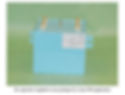
General Atomics Energy Products (GAEP) produces both individual capacitors used in PFNs, such as the plastic case units shown as an assembly for a medical accelerator application, and multiple capacitors in a single case. The unit shown here contains six individual capacitors with one common terminal, and is used in a dermatology laser application. In addition, GAEP can design and manufacture complete PFN assemblies to meet your output pulse specifications. GAEP can also produce complete pulsed power or power electronic systems.
SPECIFYING A PULSE FORMING NETWORK
Output voltage and tolerance. Note that the output voltage is half the charge voltage on the capacitors in the Type-E network.
Characteristic impedance and tolerance. The standard value is 50 ± 5 ohms. If the load impedance is not to be matched to the network impedance, define both.
Pulse Risetime is normally specified between 10% and 90% of the average pulse amplitude.
Pulse Width is normally specified as the time between the 70% average pulse amplitude points (the half power points).
Ripple is defined as the peak-to-peak voltage above and below the average peak amplitude when the PFN is discharged into a non-reactive load. Nominal design ripple value is ± 5%, and lower ripple tolerances are possible when required. Specify the maximum allowable ripple tolerance.
Pulse Decay or Fall Time (if important)
Pulse Repetition Rate and Duty Cycle are important for thermal analysis. The duty cycle should be definitively expressed in terms of seconds on and seconds off, rather than just a percentage.
Ambient Temperature Range (Operating and Storage) in °C. GAEP's standard temperature range is -35 to +65 °C, but other ranges can be accommodated.
Operating Life should be expressed in either total charge/discharge cycles or in hours of operation. (Note: GAEP will normally quote Design Life at the 90% survival reliability level unless otherwise specified.)
Mechanical requirements, including number of terminals, mounting brackets, size and weight constraints, vibration and shock requirements, etc.
Environmental conditions, including forced air circulation or natural convection, oil or pressurized gas insulation, altitude, interior or exterior installation, etc
Inductor EMF Vs. Current Flow
Interpreting Voltage & Current Waveforms


Introduction To Inductor Phasing
With the traditional way of representing a transformer, it’s pretty easy to figure out the dot convention meaning.

In the case of inductors in series AND magnetically coupled, it is not always easy to figure out if the
inductors are in phase or out of phase because they are not always represented side by side in the
traditional way of transformers.
To help us, simply “connect” the bottom of a usual transformer to follow the current and figure out what would mean in series.

In phase : Current flows in the same direction.
Out of phase: Current flows in an opposing direction.
So for 2 inductors that are magnetically coupled to each other and in series, if their input or output
currents goes in the same direction, they are in phase and if their currents oppose to each other,
they are 180° out of phase.

